


Plot3D
詳細とオプション
- Plot3Dは,曲面プロットあるいは曲面グラフとしても知られている.
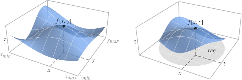
- Plot3Dは,プロットされている領域内における x と y の値のところで f を評価し,点{x,y,f[x,y]}を繋いで x および y に従って f がどのように変化するかを示す曲面を描く.
- 以下は
 の曲面を可視化する.
 - fiを評価すると実数以外になる点にはギャップが残される.
- Plot3D は,実質的にBlockを使って変数 x および y を局所的なものとして扱う.
- Plot3Dは属性HoldAllを持ち,x および y に特定の数値を割り当てた後でのみ f を評価する.
- 場合によっては,x および y に特定の数値が割り当てられる前にEvaluateを使って f を記号的に評価する方が効率的なこともある.
- fiには,次のラッパー w を使うことができる.
-
Annotation[fi,label] fiの注釈を与える Button[fi,action] fiがクリックされたときに action を評価する Callout[fi,label] 関数にコールアウトでラベルを付ける Callout[fi,label,pos] コールアウトを相対的な位置pos に置く EventHandler[fi,events] fiの一般的なイベントハンドラを定義する Hyperlink[fi,uri] 関数をハイパーリンクにする Labeled[fi,label] 関数にラベルを付ける Labeled[fi,label,pos] ラベルを相対的な位置 pos に置く Legended[fi,label] 関数を凡例で識別する PopupWindow[fi,cont] 関数にポップアップウィンドウを付ける StatusArea[fi,label] マウスオーバーの際にステータスエリアに表示する Style[fi,styles] 関数を指定のスタイルで表示する Tooltip[fi,label] 関数に任意のツールチップを付ける Tooltip[fi] 関数をツールチップとして使う - ラッパー w は複数のレベルで適用できる.
-
w[fi] fiをラップする w[{f1,…}] fiの集合をラップする w1[w2[…]] ネストしたラッパーを使う - Callout,Labeled,Placedは次の位置 pos を使うことができる.
-
Automatic 自動的に置かれたラベル Above, Below, Before, After 曲面の周囲の位置 {x,y} 位置{x,y}における曲面の近く {x,y,z} 位置{x,y,z} {s,Above},{s,Below},… 曲面近くの位置 s における相対的な位置 {pos,epos} 曲面の相対的な位置 pos に置かれたラベル内の epos - Plot3Dは,Graphics3Dと同じオプションに以下の追加・修正を加えたものが設定できる. [全オプションのリスト]
- PlotStyle->Noneは,曲面を描かないので,実質的に隠された曲面を除外することはない.
- Plot3Dはまず,PlotPointsで指定された等間隔のサンプル点の格子で各関数を評価する.次に適応的アルゴリズムを用いて,最高MaxRecursion回まで部分分割して追加的なサンプル点を選択する.
- Plot3Dは有限個のサンプル点しか使わないので,関数の特徴を見付けられない可能性もあるので注意されたい.結果の検証にはPlotPointsとMaxRecursionの設定値を大きくしてみるとよい.
- Mesh->Allの設定では,Plot3Dはすべての部分分割を表示するようにメッシュラインを描く.
- デフォルト設定のMeshFunctions->{#1&,#2&}では,x, y のメッシュが各曲面上に描かれる.
- 関数MeshFunctionsとRegionFunctionに渡される引数は x,y,zである.ColorFunctionとTextureCoordinateFunctionの関数には,デフォルトによりこれらの引数をスケールしたものが渡される.
- ColorFunction,MeshFunctions,RegionFunction,TextureCoordinateFunctionはすべて,各曲面で評価される.
- デフォルト設定のExclusions->AutomaticとExclusionsStyle->Noneでは,Plot3Dが不連続な曲線を検知すると,そこで曲面が分断される.Exclusions->Noneの場合は,不連続性があっても曲面は繋がれる.
- ScalingFunctionsの可能な設定値
-
sz z 軸をスケールする {sx,sy} x 軸と y 軸をスケールする {sx,sy,sz} x 軸,y 軸,z 軸をスケールする - 各スケーリング関数 siは,文字列"scale"か{g,g-1}である.g-1は g の逆数である.
- Plot3DはGraphics3D[GraphicsComplex[data]]を返す.
- 3D曲面に影響するテーマ
-
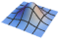
"DarkMesh" 色が濃いメッシュライン 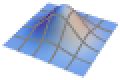
"GrayMesh" グレーメッシュライン 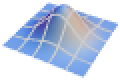
"LightMesh" 色が薄いメッシュライン 
"ZMesh" 垂直に配置されたメッシュライン 
"ThickSurface" 曲面に厚みを加える 
"FilledSurface" 曲面の下を塗り潰す
全オプションのリスト
例題
すべて開く すべて閉じる例 (4)
Plot3D[Sin[x + y ^ 2], {x, -3, 3}, {y, -2, 2}]Plot3D[{x ^ 2 + y ^ 2, -x ^ 2 - y ^ 2}, {x, -2, 2}, {y, -2, 2}, ColorFunction -> "RustTones"]Plot3D[{x ^ 2 + y ^ 2, -x ^ 2 - y ^ 2}, {x, -2, 2}, {y, -2, 2}, RegionFunction -> Function[{x, y, z}, x ^ 2 + y ^ 2 ≤ 4], BoxRatios -> Automatic]Plot3D[Im[ArcSin[(x + I y) ^ 4]], {x, -2, 2}, {y, -2, 2}, Mesh -> None, PlotStyle -> Directive[Yellow, Specularity[White, 20], Opacity[0.8]], ExclusionsStyle -> {None, Red}]スコープ (26)
サンプリング (11)
関数が急激に変化するところではより多くの点がサンプルとして取られる:
Plot3D[Sin[x y], {x, 0, 3}, {y, 0, 3}, Mesh -> All]Plot3D[1 / (x ^ 2 + y ^ 2), {x, -1, 1}, {y, -1, 1}]Plot3D[Sqrt[x y], {x, -1, 1}, {y, -1, 1}]Plot3D[Im[ArcSin[(x + I y) ^ 3]], {x, -2, 2}, {y, -2, 2}]PlotPointsとMaxRecursionを使って適応的サンプリングを制御する:
Grid[Table[Plot3D[Sin[x y], {x, 0, 4}, {y, 0, 4}, PlotPoints -> pp, MaxRecursion -> mr, Mesh -> None], {mr, {0, 1, 2}}, {pp, {5, 15}}]]PlotRangeを使って関心領域に焦点を当てる:
{Plot3D[x ^ 4 - 2x ^ 2 + y ^ 4 - 2y ^ 2 + 5, {x, -2, 2}, {y, -2, 2}], Plot3D[x ^ 4 - 2x ^ 2 + y ^ 4 - 2y ^ 2 + 1, {x, -2, 2}, {y, -2, 2}, PlotRange -> {-2, 2}, ClippingStyle -> None]}Exclusionsを使って曲線を取り除くか,または結果の曲面を分割する:
{Plot3D[1 / (ChebyshevU[x y - 1, 2]), {x, -5, 5}, {y, -5, 5}], Plot3D[1 / (ChebyshevU[x y - 1, 2]), {x, -5, 5}, {y, -5, 5}, Exclusions -> {x == 0, y == 0}]}RegionFunctionを使って曲面を不等式で与えられる領域に限定する:
Plot3D[Sin[x + y ^ 2], {x, -3, 3}, {y, -2, 2}, RegionFunction -> Function[{x, y, z}, 0 < x + y ^ 2 < Pi]]Plot3D[Sin[x + Cos[y]], {x, y}∈Disk[{0, 0}, 3]]領域はMeshRegionで指定することができる:
𝒟 = MeshRegion[{{0, 0}, {5, -2}, {3, 0}, {5, 2}}, Polygon[{1, 2, 3, 4}]];Plot3D[x ^ 2 + y ^ 2, {x, y}∈𝒟]Plot3D[ArcTan[x]ArcTan[y], {x, -Infinity, Infinity}, {y, -Infinity, Infinity}]ラベルと凡例 (6)
Labeledで曲面にラベルを付ける:
Plot3D[Labeled[Sin[x + Cos[y]], "label"], {x, -3, 3}, {y, -3, 3}]PlotLabelsで曲面にラベルを付ける:
Plot3D[Sin[x + Cos[y]], {x, -3, 3}, {y, -3, 3}, PlotLabels -> Sin[x + Cos[y]]]Plot3D[Labeled[Sin[x + Cos[y]], "label", {0, 0}], {x, -3, 3}, {y, -3, 3}]Calloutを使う:
Plot3D[Callout[Sin[x + Cos[y]], "label", {0, 0}], {x, -3, 3}, {y, -3, 3}, PlotRange -> All]Plot3D[Callout[Sin[x + Cos[y]], "label", {2, 0, 1}], {x, -3, 3}, {y, -3, 3}, PlotRange -> All]Plot3D[{x ^ 2 + y ^ 2, -x ^ 2 - y ^ 2}, {x, -2, 2}, {y, -2, 2}, PlotLegends -> "Expressions"]Legendedを使って特定の曲線に凡例を与える:
Plot3D[{x ^ 2 + y ^ 2, Legended[-x ^ 2 - y ^ 2, "surface"]}, {x, -2, 2}, {y, -2, 2}]Placedを使って凡例の位置を変える:
Plot3D[{x ^ 2 + y ^ 2, Legended[-x ^ 2 - y ^ 2, Placed["surface", Below]]}, {x, -2, 2}, {y, -2, 2}]プレゼンテーション (9)
曲面に明示的なPlotStyleを与える:
Plot3D[Sin[x + y ^ 2], {x, -2, 2}, {y, -2, 2}, PlotStyle -> Directive[Orange, Specularity[White, 20]]]Plot3D[{Sin[x], Cos[x]}, {x, 0, 2Pi}, {y, 0, 2Pi}, PlotStyle -> {Red, Blue}]Plot3D[Sin[x y], {x, 0, 3}, {y, 0, 3}, AxesLabel -> {x, y}, PlotLabel -> Sin[x y]]Plot3D[Sin[x y], {x, 0, 3}, {y, 0, 3}, ColorFunction -> Function[{x, y, z}, Hue[z]]]Plot3D[Sin[x y], {x, 0, 3}, {y, 0, 3}, ColorFunction -> "SolarColors", PlotLegends -> Automatic]Plot3D[Sin[x]Cos[y], {x, 0, 2π}, {y, 0, 2π}, PlotTheme -> "Web"]Plot3D[Sqrt[1 - x ^ 2 - y ^ 2], {x, -1, 1}, {y, -1, 1}, Mesh -> 8, ColorFunction -> Hue, MeshShading -> {{Yellow, Orange}, {Pink, Red}}]曲面にインタラクティブなTooltipを与える:
Plot3D[Tooltip[Sqrt[x y]], {x, -2, 2}, {y, -2, 2}]Plot3D[Sin[x + y ^ 2], {x, -2, 2}, {y, -2, 2}, RegionFunction -> (#1 ^ 2 + #2 ^ 2 < 4&), Filling -> Bottom, FillingStyle -> Directive[Opacity[0.4], Red]]オプション (103)
Background (1)
BoundaryStyle (6)
Plot3D[Sin[x y], {x, -2, 2}, {y, -2, 2}]Plot3D[Sin[x y], {x, -2, 2}, {y, -2, 2}, BoundaryStyle -> Thick]Plot3D[Sin[x y], {x, -2, 2}, {y, -2, 2}, BoundaryStyle -> Directive[Red, Thick]]Plot3D[Sin[x y], {x, -2, 2}, {y, -2, 2}, BoundaryStyle -> None]BoundaryStyleをRegionFunctionによって切り取られた穴に適用される:
Plot3D[Sin[x y], {x, -2, 2}, {y, -2, 2}, BoundaryStyle -> Thick, RegionFunction -> Function[{x, y, z}, x ^ 2 + y ^ 2 ≥ 1]]BoundaryStyleはExclusionsによって切り取られた穴には適用されない:
Plot3D[Im[Sqrt[x + I y]], {x, -2, 2}, {y, -2, 2}, BoundaryStyle -> Thick]BoxRatios (2)
AutomaticはPlotRangeの自然なスケールを使用する:
{Plot3D[Sqrt[1 - x ^ 2 - y ^ 2], {x, 0, 1}, {y, 0, 1}], Plot3D[Sqrt[1 - x ^ 2 - y ^ 2], {x, 0, 1}, {y, 0, 1}, BoxRatios -> Automatic]}BoxRatiosを使って特定の特徴を強調する.この場合は鞍部の曲面が強調されている:
Plot3D[y ^ 2 - x ^ 2, {x, -4, 4}, {y, -4, 4}, MeshFunctions -> {#3&}, BoxRatios -> {1, 1, 2}]ClippingStyle (4)
切り取られた部分には,デフォルトで,異なる曲面の色が用いられる:
Plot3D[Re[Sin[x + I y]], {x, -2Pi, 2Pi}, {y, -2Pi, 2Pi}]Plot3D[Re[Sin[x + I y]], {x, -2Pi, 2Pi}, {y, -2Pi, 2Pi}, ClippingStyle -> None]Plot3D[Re[Sin[x + I y]], {x, -2Pi, 2Pi}, {y, -2Pi, 2Pi}, ClippingStyle -> Opacity[0.5]]Plot3D[Re[Sin[x + I y]], {x, -2Pi, 2Pi}, {y, -2Pi, 2Pi}, ClippingStyle -> {Red, Blue}]ColorFunction (6)


Plot3D[Sin[x y], {x, 0, 3}, {y, 0, 3}, ColorFunction -> Function[{x, y, z}, RGBColor[x, y, 0.]]]
Plot3D[x / Exp[x ^ 2 + y ^ 2], {x, -2, 2}, {y, -2, 2}, ColorFunction -> Function[{x, y, z}, Hue[.65(1 - z)]]]定義済みの色階調度にColorDataを使う:
Plot3D[x / Exp[x ^ 2 + y ^ 2], {x, -2, 2}, {y, -2, 2}, ColorFunction -> (ColorData["DarkRainbow"][#3]&)]
Plot3D[x / Exp[x ^ 2 + y ^ 2], {x, -2, 2}, {y, -2, 2}, ColorFunction -> "DarkRainbow"]ColorFunctionはPlotStyleより優先順位が高い:
Plot3D[x / Exp[x ^ 2 + y ^ 2], {x, -2, 2}, {y, -2, 2}, ColorFunction -> "DarkRainbow", PlotStyle -> Directive[Opacity[0.5], Red]]ColorFunctionはMeshShadingより優先順位が低い:
Plot3D[x / Exp[x ^ 2 + y ^ 2], {x, -2, 2}, {y, -2, 2}, ColorFunction -> Hue, MeshShading -> {{Automatic, None}, {None, Automatic}}]ColorFunctionScaling (2)
Plot3D[Abs[Sin[x + I y]], {x, -2Pi, 2Pi}, {y, -2, 2}, ColorFunction -> Function[{x, y, z}, Hue@Rescale[Arg[Sin[x + I y]], {-Pi, Pi}]], ColorFunctionScaling -> False] 方向にはスケールされた座標を,
 方向と
方向と  方向にはスケールされていない座標を使う:
Plot3D[Sin[x y], {x, 0, 3}, {y, 0, 3}, ColorFunction -> Function[{x, y, z}, Hue[y, x, 1]], ColorFunctionScaling -> {True, False, False}]EvaluationMonitor (2)
Plot3Dがどこで関数をサンプルするかを示す:
ListPlot[Reap[Plot3D[Sin[x]Sin[y], {x, -2, 2}, {y, -3, 3}, EvaluationMonitor :> Sow[{x, y}]]][[-1, 1]]]
Block[{k = 0}, Plot3D[Sin[x y], {x, 0, 2}, {y, 0, 2}, EvaluationMonitor :> k++];k]Exclusions (5)
これは自動のメソッドを使って除外するものを,この場合は分枝切断線から,計算する:
Plot3D[Im[ArcSin[x + I y]], {x, -2, 2}, {y, -2, 2}]Plot3D[Im[ArcSin[x + I y]], {x, -2, 2}, {y, -2, 2}, Exclusions -> None]Plot3D[1 / (ChebyshevU[x y - 1, 2]), {x, -2, 2}, {y, -2, 2}, Exclusions -> {x == 0, y == 0}]Plot3D[Im[Sqrt[x + I y]], {x, -2, 2}, {y, -2, 2}, Exclusions -> {{y == 0, x ≤ 0}}]Plot3D[Im[Sqrt[I x y] / (ChebyshevU[x ^ 2 - y ^ 2, 2])], {x, -2, 2}, {y, -2, 2}, Exclusions -> {Automatic, y ^ 2 - x ^ 2 == 1}]ExclusionsStyle (3)
Plot3D[Im[ArcSin[x + I y]], {x, -2, 2}, {y, -2, 2}, ExclusionsStyle -> {None, Directive[Thick, Blue]}]Plot3D[Im[ArcSin[x + I y]], {x, -2, 2}, {y, -2, 2}, ExclusionsStyle -> {Opacity[0.5], Directive[Thick, Blue]}]Plot3D[Im[ArcSin[x + I y]], {x, -2, 2}, {y, -2, 2}, ExclusionsStyle -> Opacity[0.5]]Filling (4)
Plot3D[Sin[x + y ^ 2], {x, -2, 2}, {y, -2, 2}, Filling -> Bottom]RegionFunctionによって切り取られた領域に沿って塗潰しが行われる:
Plot3D[Sin[x + y ^ 2], {x, -2, 2}, {y, -2, 2}, Filling -> Bottom, RegionFunction -> (#1 ^ 2 + #2 ^ 2 < 3&)]Plot3D[Sin[x + y ^ 2], {x, -2, 2}, {y, -2, 2}, Filling -> {1 -> Top, 1 -> Bottom}, RegionFunction -> (#1 ^ 2 + #2 ^ 2 < 3&)]Plot3D[{Cos[x], Cos[x] + 1}, {x, 0, 2Pi}, {y, 0, 2Pi}, Filling -> {1 -> {Bottom, Blue}, 2 -> {Top, Red}}]FillingStyle (3)
Table[Plot3D[Sin[x + y ^ 2], {x, -2, 2}, {y, -2, 2}, Filling -> Bottom, FillingStyle -> fs], {fs, {Opacity[0.5], Orange}}]
Plot3D[Sin[x + y ^ 2], {x, -2, 2}, {y, -2, 2}, Filling -> 0, FillingStyle -> {Red, Blue}]
Plot3D[Sin[x + y ^ 2], {x, -2, 2}, {y, -2, 2}, Filling -> 0, FillingStyle -> {Red, None}]LabelingSize (2)
Plot3D[Sin[x + Cos[y]], {x, 0, 5}, {y, 0, 5}, PlotLabels -> "tropopause"]Plot3D[Sin[x + Cos[y]], {x, 0, 5}, {y, 0, 5}, PlotLabels -> "tropopause", LabelingSize -> 30]label = [image];Plot3D[Sin[x + Cos[y]], {x, 0, 5}, {y, 0, 5}, PlotLabels -> label]Plot3D[Sin[x + Cos[y]], {x, 0, 5}, {y, 0, 5}, PlotLabels -> label, LabelingSize -> 60]Plot3D[Sin[x + Cos[y]], {x, 0, 5}, {y, 0, 5}, PlotLabels -> label, LabelingSize -> Full]MaxRecursion (1)
Mesh (6)
Plot3D[Sin[x + y ^ 2], {x, -3, 3}, {y, -2, 2}, Mesh -> None]{Plot3D[Sin[x + y ^ 2], {x, -3, 3}, {y, -2, 2}, Mesh -> Full], Plot3D[Sin[x + y ^ 2], {x, -3, 3}, {y, -2, 2}, Mesh -> All]}Plot3D[Sin[x + y ^ 2], {x, -3, 3}, {y, -2, 2}, Mesh -> 5] 方向に3本のメッシュライン,
 方向に6本のメッシュラインを使う:
Plot3D[Sin[x + y ^ 2], {x, -3, 3}, {y, -2, 2}, Mesh -> {3, 6}]Plot3D[Sin[x + y ^ 2], {x, -3, 3}, {y, -2, 2}, Mesh -> {{-1, 1}, {0}}]Plot3D[Sin[x + y ^ 2], {x, -3, 3}, {y, -2, 2}, Mesh -> {{{0, Thick}}, {{0, Red}}}]MeshFunctions (3)

Plot3D[Sin[x + y ^ 2], {x, -3, 3}, {y, -2, 2}, MeshFunctions -> {#3&}, Mesh -> 5]

Plot3D[Sin[x + y ^ 2], {x, -3, 3}, {y, -2, 2}, MeshFunctions -> {#1&, #2&}, Mesh -> {5, 5}]Plot3D[Sin[x + y ^ 2], {x, -3, 3}, {y, -2, 2}, MeshFunctions -> {Sqrt[#1 ^ 2 + #2 ^ 2 + #3 ^ 2]&}, Mesh -> 5]MeshShading (4)
Noneを使って領域を取り除く:
Plot3D[Sin[x y], {x, 0, 3}, {y, 0, 3}, Mesh -> 10, MeshFunctions -> {#3&}, MeshShading -> {Red, None}]Plot3D[Sin[x y], {x, 0, 3}, {y, 0, 3}, Mesh -> 7, MeshFunctions -> {#1&, #2&}, MeshShading -> {{Yellow, Green}, {Green, Yellow}}]MeshShadingはPlotStyleより優先順位が高い:
Plot3D[Sin[x y], {x, 0, 3}, {y, 0, 3}, Mesh -> 7, PlotStyle -> Red, MeshShading -> {{Automatic, Green}, {Green, Automatic}}]MeshShadingはColorFunctionより優先順位が高い:
Plot3D[Sin[x y], {x, 0, 3}, {y, 0, 3}, Mesh -> 10, MeshFunctions -> {#1&, #2&}, MeshShading -> {{Automatic, None}, {None, Automatic}}, ColorFunction -> "DarkRainbow"]MeshStyle (2)


NormalsFunction (3)
Plot3D[Sin[x + y ^ 2], {x, -3, 3}, {y, -2, 2}, Mesh -> None]Noneを使ってすべての多角形に平坦な陰影付けを施す:
Plot3D[Sin[x + y ^ 2], {x, -3, 3}, {y, -2, 2}, NormalsFunction -> None, Mesh -> None]Plot3D[Sin[x + y ^ 2], {x, -3, 3}, {y, -2, 2}, Mesh -> None, NormalsFunction -> Function[{x, y, z}, RandomReal[{0, 1}, {3}]]]PerformanceGoal (2)
PlotLabels (3)
Plot3D[-x ^ 2 - y ^ 2, {x, -2, 2}, {y, -2, 2}, PlotLabels -> "Expressions"]Plot3D[-x ^ 2 - y ^ 2, {x, -2, 2}, {y, -2, 2}, PlotLabels -> "paraboloid"]Plot3D[{x ^ 2 + y ^ 2, -x ^ 2 - y ^ 2}, {x, 0, 2}, {y, -2, 2}, PlotLabels -> {Callout["label1", Above], Callout["label2", Below]}]PlotLegends (5)
Plot3D[{Sin[x^2 + y], Cos[x^2 + y]}, {x, 0, Pi}, {y, 0, Pi}, PlotLegends -> Automatic]Plot3D[{Sin[x^2 + y], Cos[x^2 + y]}, {x, 0, Pi}, {y, 0, Pi}, PlotLegends -> {"one", "two"}]Plot3D[{Sin[x^2 + y], Cos[x^2 + y]}, {x, 0, Pi}, {y, 0, Pi}, PlotLegends -> "Expressions"]Placedを使って凡例の位置を制御する:
Plot3D[{Sin[x^2 + y], Cos[x^2 + y]}, {x, 0, Pi}, {y, 0, Pi}, PlotLegends -> Placed[Automatic, Below]]SwatchLegendを使って外観を変える:
Plot3D[{Sin[x^2 + y], Cos[x^2 + y]}, {x, 0, Pi}, {y, 0, Pi}, PlotLegends -> SwatchLegend[Automatic, {"surf1", "surf2"}, LegendFunction -> "Frame", LegendMargins -> 10]]Plot3D[Sin[x^2 + y], {x, 0, Pi}, {y, 0, Pi}, ColorFunction -> "Rainbow", PlotLegends -> Automatic]BarLegendを使って外観を変える:
Plot3D[Sin[x^2 + y], {x, 0, Pi}, {y, 0, Pi}, ColorFunction -> "Rainbow", PlotLegends -> BarLegend[Automatic, LegendMarkerSize -> {10, 100}]]PlotPoints (2)
Table[Plot3D[Sin[x + y ^ 2], {x, -3, 3}, {y, -2, 2}, Mesh -> None, MaxRecursion -> 0, PlotPoints -> pp], {pp, {5, 10, 15, 20}}]

Plot3D[Sin[2x]y, {x, 0, 2Pi}, {y, -1, 1}, PlotPoints -> {20, 5}, Mesh -> Full]PlotRange (5)

Plot3D[1 / (x ^ 2 + y ^ 2), {x, -2, 2}, {y, -2, 2}]Plot3D[1 / (x ^ 2 + y ^ 2), {x, -2, 2}, {y, -2, 2}, PlotRange -> All]

Plot3D[Sqrt[1 - x ^ 2 - y ^ 2], {x, -2, 2}, {y, -2, 2}, PlotRange -> Full]

Plot3D[Sqrt[1 - x ^ 2 - y ^ 2], {x, -2, 2}, {y, -2, 2}, PlotRange -> Automatic]
Plot3D[x ^ 2 - y ^ 2, {x, -4, 4}, {y, -4, 4}, PlotRange -> {-2, 2}]PlotStyle (5)
Plot3D[Sin[x + y ^ 2], {x, -3, 3}, {y, -2, 2}, PlotStyle -> Orange]Specularityを使ってハイライトする:
Plot3D[Sin[x + y ^ 2], {x, -3, 3}, {y, -2, 2}, PlotStyle -> Directive[Orange, Specularity[White, 50]]]Opacityを使って透過的な曲面を得る:
Plot3D[Sin[x + y ^ 2], {x, -3, 3}, {y, -2, 2}, PlotStyle -> Directive[Opacity[0.8], Orange, Specularity[White, 50]]]Plot3D[{Re[Sin[x + I y]], Im[Sin[x + I y]]}, {x, -2Pi, 2Pi}, {y, -2Pi, 2Pi}, PlotStyle -> {Red, Blue}]Plot3D[Sin[x + y ^ 2], {x, -3, 3}, {y, -2, 2}, PlotStyle -> None]PlotTheme (2)
Plot3D[{4 + x ^ 2 - y ^ 2, -4 - x ^ 2 + y ^ 2}, {x, -2, 2}, {y, -2, 2}, PlotTheme -> "Detailed"]Plot3D[{4 + x ^ 2 - y ^ 2, -4 - x ^ 2 + y ^ 2}, {x, -2, 2}, {y, -2, 2}, PlotTheme -> "Detailed", FaceGrids -> None]Plot3D[Sin[x], {x, 0, 2Pi}, {y, 0, π / 2}, PlotTheme -> "ThickSurface"]RegionFunction (4)


Plot3D[Sin[x + y ^ 2], {x, -2, 2}, {y, -2, 2}, RegionFunction -> Function[{x, y, z}, 2 < x ^ 2 + y ^ 2 < 5]]Fillingは領域境界から塗り潰す:
Plot3D[Sin[x + y ^ 2], {x, -2, 2}, {y, -2, 2}, RegionFunction -> Function[{x, y, z}, 2 < x ^ 2 + y ^ 2 < 5], Filling -> Bottom]Plot3D[Sin[x + y ^ 2], {x, -2, 2}, {y, -2, 2}, RegionFunction -> Function[{x, y, z}, 0 < Mod[x ^ 2 + y ^ 2, 2] < 1]]Plot3D[Exp[-(x ^ 2 + y ^ 2)], {x, -2, 2}, {y, -2, 2}, RegionFunction -> Function[{x, y, z}, x < 0 || y > 0]]ScalingFunctions (9)
Plot3D[Max[x, y], {x, 0, 10}, {y, 0, 10}]
Plot3D[Max[x, y], {x, 0, 10}, {y, 0, 10}, ScalingFunctions -> "Log"]
Plot3D[Max[x, y], {x, 0, 10}, {y, 0, 10}, ScalingFunctions -> "Reverse"]
Plot3D[Max[x, y], {x, 0, 10}, {y, 0, 10}, ScalingFunctions -> "Reciprocal"]

Plot3D[Max[x, y], {x, 0, 10}, {y, 0, 10}, ScalingFunctions -> {"Reverse", "Log"}]

Plot3D[Max[x, y], {x, 0, 10}, {y, 0, 10}, ScalingFunctions -> {"Reverse", None}]Plot3D[Max[x, y], {x, 0, 10}, {y, 0, 10}, ScalingFunctions -> {{-Log[#]&, Exp[-#]&}, None}]Ticksの中の位置は自動的にスケールされる:
Plot3D[x ^ 2 + y ^ 2, {x, 0, 10}, {y, 0, 10}, ScalingFunctions -> {"Log", None, None}, Ticks -> {2 ^ Range[10], Automatic, Automatic}]PlotRangeは自動的にスケールされる:
Plot3D[x ^ 2 + y ^ 2, {x, 0, 10}, {y, 0, 10}, ScalingFunctions -> "Log", PlotRange -> {1, 100}]TextureCoordinateFunction (4)


Plot3D[Sin[x y], {x, 0, 3}, {y, 0, 3}, Mesh -> None, PlotStyle -> Texture[ExampleData[{"ColorTexture", "MultiSpiralsPattern"}]]]

Plot3D[Sin[x y], {x, 0, 3}, {y, 0, 3}, Mesh -> None, TextureCoordinateFunction -> ({#1, #3}&), PlotStyle -> Texture[ExampleData[{"ColorTexture", "MultiSpiralsPattern"}]]]Plot3D[Sin[x y], {x, 0, 3}, {y, 0, 3}, Mesh -> None, TextureCoordinateScaling -> False, PlotStyle -> Texture[ExampleData[{"ColorTexture", "MultiSpiralsPattern"}]]]テクスチャを使ってパラメータがどのように曲面にマップされるかをハイライトする:
texture = ArrayPlot[{{1, 1, 1, 2, 1, 1}, {2, 0, 0, 2, 0, 0}, {2, 0, 0, 2, 0, 0}, {2, 1, 1, 1, 1, 1}, {2, 0, 0, 2, 0, 0}, {2, 0, 0, 2, 0, 0}}, ColorRules -> {1 -> Red, 2 -> Blue, 0 -> White}, Frame -> False, PlotRangePadding -> None, ImagePadding -> None, ImageSize -> 100]Plot3D[Sin[x y], {x, 0, 3}, {y, 0, 3}, Mesh -> None, TextureCoordinateScaling -> False, PlotStyle -> Texture[texture]]TextureCoordinateScaling (1)
テクスチャにスケールされたあるいはスケールされていない座標を使う:
texture = ArrayPlot[{{1, 1, 1, 2, 1, 1}, {2, 0, 0, 2, 0, 0}, {2, 0, 0, 2, 0, 0}, {2, 1, 1, 1, 1, 1}, {2, 0, 0, 2, 0, 0}, {2, 0, 0, 2, 0, 0}}, ColorRules -> {1 -> Red, 2 -> Blue, 0 -> White}, Frame -> False, PlotRangePadding -> None, ImagePadding -> None, ImageSize -> 100]Table[Plot3D[Sin[x y], {x, 0, 3}, {y, 0, 3}, Mesh -> None, TextureCoordinateScaling -> s, PlotStyle -> Texture[texture], PlotLabel -> s], {s, {True, False}}]アプリケーション (17)
基本的なアプリケーション (7)
Plot3D[ (x^2 + y^2) Exp[1 - x^2 - y^2], {x, -3, 3}, {y, -3, 3}, PlotStyle -> Opacity[0.5], Mesh -> None, PlotPoints -> 50]内部構造が見えるように,MeshShadingを使って表面に穴を開ける:
Plot3D[ (x^2 + y^2) Exp[1 - x^2 - y^2], {x, -3, 3}, {y, -3, 3}, MeshShading -> {{Automatic, None}, {None, Automatic}}, PlotPoints -> 50]MeshFunctionsを使って使用するスライスも指定する:
Plot3D[ (x^2 + y^2) Exp[1 - x^2 - y^2], {x, -3, 3}, {y, -3, 3}, MeshFunctions -> {#3&}, Mesh -> 8, MeshShading -> {Automatic, None}, PlotPoints -> 50]


Plot3D[{x^2 + y^2, x^2 - y^2}, {x, -1, 1}, {y, -1, 1}, BoxRatios -> Automatic, PlotLegends -> "Expressions"]Simplify[x^2 - y^2 ≤ x^2 + y^2, {x, y}∈Reals]![TemplateBox[{p, infty}, Norm2]<=TemplateBox[{p, 2}, Norm2]<=TemplateBox[{p, 1}, Norm2]](Files/Plot3D.ja/2.png "TemplateBox[{p, infty}, Norm2]<=TemplateBox[{p, 2}, Norm2]<=TemplateBox[{p, 1}, Norm2]")
Plot3D[{Norm[{x, y}, 1], Norm[{x, y}, 2], Norm[{x, y}, ∞]}, {x, -1, 1}, {y, -1, 1}, PlotStyle -> Opacity[0.7], Mesh -> None, PlotLegends -> "Expressions"]Simplify[Norm[{x, y}, ∞] ≤ Norm[{x, y}, 2] ≤ Norm[{x, y}, 1], {x, y}∈Reals]knots = {0, 0, 0, 1 / 2, 1, 1, 1};
fx = Table[BSplineBasis[{2, knots}, i, x], {i, 0, 3}];
fy = Table[BSplineBasis[{2, knots}, i, y], {i, 0, 3}];
fxy = Times@@@Tuples[{fx, fy}];Plot3D[Evaluate@fxy, {x, 0, 1}, {y, 0, 1}, PlotRange -> All, PlotPoints -> 50, PlotLegends -> "Expressions"]


Table[Plot3D[Norm[{x, y}, p], {x, -1.5, 1.5}, {y, -1.5, 1.5}, Ticks -> None, MeshFunctions -> {#3&}, Mesh -> {{1}}, MeshStyle -> Dashed, PlotLabel -> Norm[x, p]], {p, {1, 2, 3, Infinity}}]鞍部曲面をプロットする.メッシュ曲線は関数が零になるところを示している:
Plot3D[y ^ 2 - x ^ 2, {x, -4, 4}, {y, -4, 4}, MeshFunctions -> {#3&}, Mesh -> {{0}}, BoxRatios -> 1]関数の特徴 (2)
RegionFunctionを使って極限の動作を理解するための切り出しを作る:
Plot3D[(10 x y/2x^2 + 3y^2), {x, -3, 3}, {y, -3, 3}, RegionFunction -> Function[{x, y, z}, 2x^2 + 3y^2 > 1 / 5], Mesh -> None]{Limit[(10 x y/2x^2 + 3y^2), x -> y], Limit[(10 x y/2x^2 + 3y^2), x -> -y]}MeshFunctionsを使って関数  の極値をハイライトする:
f = Sin[Sqrt[2]x + y] + Sin[y];Plot3D[f, {x, 0, 10}, {y, 0, 10}, Mesh -> None]

mfx = Function[{x, y, z}, Evaluate[D[f, x]]];Plot3D[f, {x, 0, 10}, {y, 0, 10}, MeshFunctions -> {mfx}, Mesh -> {{0}}, MeshStyle -> {{Red}}, PlotPoints -> 50]

mfy = Function[{x, y, z}, Evaluate[D[f, y]]];Plot3D[f, {x, 0, 10}, {y, 0, 10}, MeshFunctions -> {mfy}, Mesh -> {{0}}, MeshStyle -> {{Blue}}, PlotPoints -> 50]

Plot3D[f, {x, 0, 10}, {y, 0, 10}, MeshFunctions -> {mfx, mfy}, Mesh -> {{0}, {0}}, MeshStyle -> {{Red}, {Blue}}, PlotPoints -> 50]勾配磁場 (2)
s = StreamPlot[Evaluate@Grad[Sin[x + y ^ 2], {x, y}], {x, -3, 3}, {y, -2, 2}, Frame -> False, PlotRangePadding -> None];Plot3D[Sin[x + y ^ 2], {x, -3, 3}, {y, -2, 2}, PlotStyle -> Texture[s], Mesh -> None]v = VectorPlot[Evaluate@Grad[Sin[x + y ^ 2], {x, y}], {x, -3, 3}, {y, -2, 2}, Frame -> False, PlotRangePadding -> None];Plot3D[Sin[x + y ^ 2], {x, -3, 3}, {y, -2, 2}, PlotStyle -> Texture[v], Mesh -> None]エピグラフとハイポグラフ (2)
関数  のエピグラフは
 で与えられる.Fillingを使ってこれを可視化することができる:
Plot3D[Sin[x + y ^ 2], {x, -3, 3}, {y, -2, 2}, Filling -> {1 -> Top}, PlotRange -> 2]関数  のハイポグラフは
 で与えられる.Fillingを使ってこれを可視化することができる:
Plot3D[Sin[x + y ^ 2], {x, -3, 3}, {y, -2, 2}, Filling -> {1 -> Bottom}, PlotRange -> 2]複素関数 (2)

Plot3D[{Re[Sin[x + I y]], Im[Sin[x + I y]]}, {x, -2Pi, 2Pi}, {y, 0, 2}, BoxRatios -> Automatic, Ticks -> {Range[-2Pi, 2Pi, Pi], {0, 1, 2}}, Mesh -> None, PlotStyle -> {Yellow, Cyan}, AxesLabel -> Automatic]Table[Plot3D[f[ArcSin[(x + I y) ^ 2]], {x, -2, 2}, {y, -2, 2}, Mesh -> None, PlotStyle -> Directive[Yellow, Specularity[White, 20], Opacity[0.8]], ExclusionsStyle -> {None, Red}], {f, {Re, Im, Abs, Arg}}]その他のアプリケーション (2)
NDSolve[{D[u[t, x], t] == D[u[t, x], x, x], u[0, x] == 0, u[t, 0] == Sin[t], u[t, 5] == 0}, u, {t, 0, 10}, {x, 0, 5}]Plot3D[Evaluate[u[t, x] /. %], {t, 0, 10}, {x, 0, 5}, PlotRange -> All, ColorFunction -> "SunsetColors"]反復するロジスティック写像をパラメータと初期値の関数としてプロットする:
Plot3D[Nest[a #(1 - #)&, x0, 100], {a, 0, 3.6}, {x0, 0.1, 0.9}, AxesLabel -> Automatic]特性と関係 (8)
Plot3Dは,必要な場合はより多くの点をサンプルとして取る:
Plot3D[Sin[x y], {x, 0, 3}, {y, 0, 3}, Mesh -> All]Plot3DはParametricPlot3Dの特殊ケースである:
{Plot3D[Sin[x y], {x, -2, 2}, {y, -2, 2}], ParametricPlot3D[{x, y, Sin[x y]}, {x, -2, 2}, {y, -2, 2}, BoxRatios -> {1, 1, 0.4}]}データのプロットにListPlot3Dを使う:
data = Table[Sin[x y], {x, 0, 3, .1}, {y, 0, 3, .1}];ListPlot3D[data]ComplexPlot3Dは,関数の大きさを位相を使って高さと色としてプロットする:
ComplexPlot3D[Sin[z] ^ 3 / (z + 1) ^ 4, {z, -5 - 5I, 5 + 5I}]Plot3D[Abs[Sin[x + I * y] ^ 3 / (x + I * y + 1) ^ 4], {x, -5, 5}, {y, -5, 5}]Plotを一変量関数に使う:
Plot[Sin[x] + Sin[Sqrt[2]x], {x, 0, 20}]ParametricPlotを平面のパラメトリック曲線と範囲に使う:
{ParametricPlot[{Cos[θ], Sin[θ]}, {θ, 0, 2Pi}], ParametricPlot[{r Cos[θ], r Sin[θ]}, {θ, 0, 2Pi}, {r, 1 / 2, 1}]}ContourPlot3DとRegionPlot3Dを陰的な曲面と範囲に使う:
{ContourPlot3D[Sin[x y] == z, {x, -2, 2}, {y, -2, 2}, {z, -2, 2}],
RegionPlot3D[Sin[x y] ≥ z, {x, -2, 2}, {y, -2, 2}, {z, -2, 2}]}DensityPlotとContourPlotを密度と等高線に使う:
{DensityPlot[Sin[x y], {x, -2, 2}, {y, -2, 2}],
	ContourPlot[Sin[x y], {x, -2, 2}, {y, -2, 2}]}
おもしろい例題 (2)
$InverseTrigFunctions = {ArcSin, ArcCos, ArcSec, ArcCsc, ArcTan, ArcCot, ArcSinh, ArcCosh, ArcSech, ArcCsch, ArcTanh, ArcCoth};Table[Plot3D[Im[f[(x + I y) ^ 3]], {x, -2, 2}, {y, -2, 2}, PlotStyle -> Directive[Pink, Specularity[White, 50], Opacity[0.8]], ExclusionsStyle -> {None, Red}, ClippingStyle -> None, Mesh -> None, PlotLabel -> Im[f[(x + I y) ^ 3]], Ticks -> None], {f, $InverseTrigFunctions}]$TrigFunctions = {Sin, Cos, Sec, Csc, Tan, Cot, ArcSin, ArcCos, ArcSec, ArcCsc, ArcTan, ArcCot, Sinh, Cosh, Sech, Csch, Tanh, Coth, ArcSinh, ArcCosh, ArcSech, ArcCsch, ArcTanh, ArcCoth};Table[Plot3D[Abs[f[x + I y]], {x, -2, 2}, {y, -2, 2}, MeshFunctions -> Function@@@{{{x, y, z}, Re[f[x + I y]]}, {{x, y, z}, Im[f[x + I y]]}}, MeshStyle -> {Orange, Green}, PlotLabel -> f, Ticks -> None], {f, $TrigFunctions}]
 プログラミングの基本:グラフィックス
 NKS|Online
テキスト
Wolfram Research (1988), Plot3D, Wolfram言語関数, https://reference.wolfram.com/language/ref/Plot3D.html (2021年に更新).
CMS
Wolfram Language. 1988. "Plot3D." Wolfram Language & System Documentation Center. Wolfram Research. Last Modified 2021. https://reference.wolfram.com/language/ref/Plot3D.html.
APA
Wolfram Language. (1988). Plot3D. Wolfram Language & System Documentation Center. Retrieved from https://reference.wolfram.com/language/ref/Plot3D.html